Calibrated Test-Time Guidance for Bayesian Inference

Daniel Geyfman*, Felix Draxler*, Jan Groeneveld*, Hyunsoo Lee, Theofanis Karaletsos, Stephan Mandt

ICML 2026

Test-time guidance turns a pretrained diffusion model into a reusable prior, solving a wide variety of tasks without training a conditional model. At inference time, we combine it with a new likelihood, reward, or physics constraint that may not have been available during training. Calibrated Bayesian Guidance (CBG) gives consistent estimators for sampling the resulting Bayesian diffusion posterior instead of just optimizing reward.

Overview figure for Calibrated Bayesian Guidance

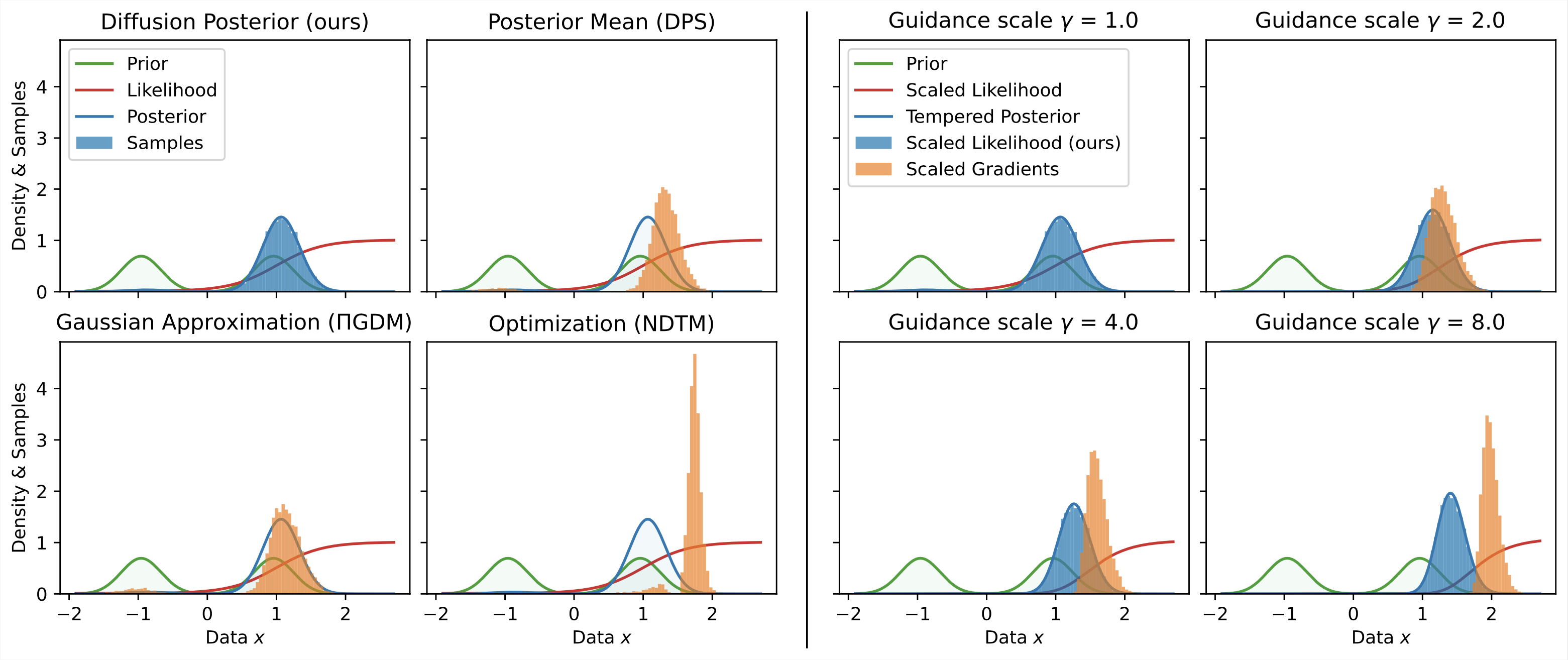
(Left) CBG estimators recover the Bayesian posterior, while common guidance approximations are biased.
(Right) CBG applies the guidance scale inside the diffused likelihood, avoiding the bias caused by naively rescaling noisy gradients.

Test-Time Guidance as Bayesian Inference

Many scientific inverse problems are too specialized to train a new conditional generative model for every measurement process. Test-time guidance solves this by reusing a pretrained diffusion model as a prior \(p(x)\), then injecting a task-specific likelihood or reward only at sampling time.

At the clean-data level, the target posterior is \[ p(x \mid y) \propto p(x)\,p(y \mid x), \qquad p(y \mid x) \propto \exp(r(x; y)). \] Along the diffusion trajectory, this induces a posterior over the noisy state \(x_t\): \[ p(x_t \mid y) \propto p(x_t)\,p(y \mid x_t), \qquad p(y \mid x_t) = \int p(x \mid x_t)\,p(y \mid x)\,dx. \] Here \(p(x \mid x_t)\) is the denoising distribution from the forward noising process. It is not the task-conditioned Bayesian posterior; the observation \(y\) enters through the likelihood weights.

Gradient-free CBG samples clean candidates from \(p(x \mid x_t)\), scores them with \(p(y \mid x)\), and uses a likelihood-weighted average to guide the next denoising step. The animation shows \(K=3\) candidates for illustration.

The Guidance Gradient of the Bayesian Posterior

Bayes' rule gives the score needed by a guided diffusion sampler: \[ \nabla_{x_t}\log p(x_t \mid y) = \underbrace{\nabla_{x_t}\log p(x_t)}_{\text{pretrained diffusion prior}} + \underbrace{\nabla_{x_t}\log p(y \mid x_t)}_{\text{guidance term}}. \] The first term is already learned by the pretrained diffusion model. The hard part is the diffused likelihood gradient, because \(p(y \mid x_t)\) averages the clean-data likelihood over all plausible denoisings of \(x_t\).

CBG estimates this term with the REINFORCE identity. After simplifying with the Gaussian forward process \(p(x_t \mid x)=\mathcal{N}(x_t; a_t x, b_t^2 I)\), the gradient-free estimator is particularly simple: \[ \nabla_{x_t}\log p(x_t \mid y) \approx \frac{\sum_{i=1}^{K} w_i\,\frac{a_t x^{(i)} - x_t}{b_t^2}} {\sum_{i=1}^{K} w_i}, \qquad x^{(i)} \sim p(x \mid x_t), \quad w_i = p(y \mid x^{(i)}). \] This requires only likelihood evaluations, so it also works for black-box or non-differentiable rewards. For differentiable rewards, CBG also admits a reparameterization-gradient estimator; see the paper for the full derivation.

Why Standard Guidance Can Fail

The calibrated guidance term depends on the true diffused likelihood \[ p(y \mid x_t) = \int p(x \mid x_t)p(y \mid x)dx. \] Many existing methods avoid this integral by replacing the denoising distribution \(p(x \mid x_t)\) with a point estimate, such as \(\mathbb{E}[x \mid x_t]\), or with a Gaussian proxy. These approximations can be useful for reward maximization, but they are biased for posterior sampling: more compute can reduce variance while still converging to the wrong distribution.

The same issue appears when using a guidance scale \(\gamma\). For calibrated tempered inference, the target is \[ p(x \mid y, \gamma) \propto p(x)p(y \mid x)^\gamma. \] Therefore the scaled likelihood must be diffused as \[ p(y \mid x_t, \gamma) \propto \int p(x \mid x_t)p(y \mid x)^\gamma dx, \] rather than by simply multiplying \(\nabla_{x_t}\log p(y \mid x_t)\) by \(\gamma\). CBG puts the likelihood, reward, and guidance scale inside the same expectation, which is what makes the resulting sampler calibrated.
Fast Sampling

CBG relies on candidate clean samples from the denoising distribution \(p(x \mid x_t)\) at each step. With analytic priors and likelihoods, this distribution can sometimes be sampled in closed form. For images and other high-dimensional scientific data, running a full inner diffusion sampler for every candidate would be too expensive.

To make CBG practical, we use one-step or few-step models to approximate these candidates. In particular, a deterministic one-step or few-step denoiser \(x=f_t(x_t)\) can be turned into a stochastic candidate generator by renoising: \[ x^{(i)} = f_t\!\left(a_t f_t(x_t) + b_t\epsilon^{(i)}\right), \qquad \epsilon^{(i)} \sim \mathcal{N}(0, I). \] This reduces the cost to draw the intermediate samples by several orders of magnitude compared to drawing samples from a diffusion model.

Renoising generates diverse candidate samples from a fast deterministic model. The animation shows \(K=3\) candidates for illustration.

Benchmarking CBG

Across several diverse benchmarks, CBG gives better calibrated posterior samples than other test-time guidance methods, and improves as the likelihood-evaluation budget increases.

Bayesian Inference

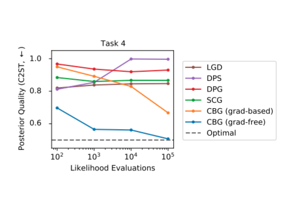
On five Bayesian inverse-problem benchmarks with reference samples from the true posterior, CBG improves distributional accuracy as the likelihood-evaluation budget increases. Both gradient-free and gradient-based CBG move toward the optimal C2ST value, while other test-time guidance methods generally plateau because their diffused-likelihood approximations remain biased.

Bayesian inference benchmark results
Task 4 from the Bayesian inverse problems benchmark. CBG visibly outperforms other methods and converges to the correct distribution.

Black-Hole Imaging

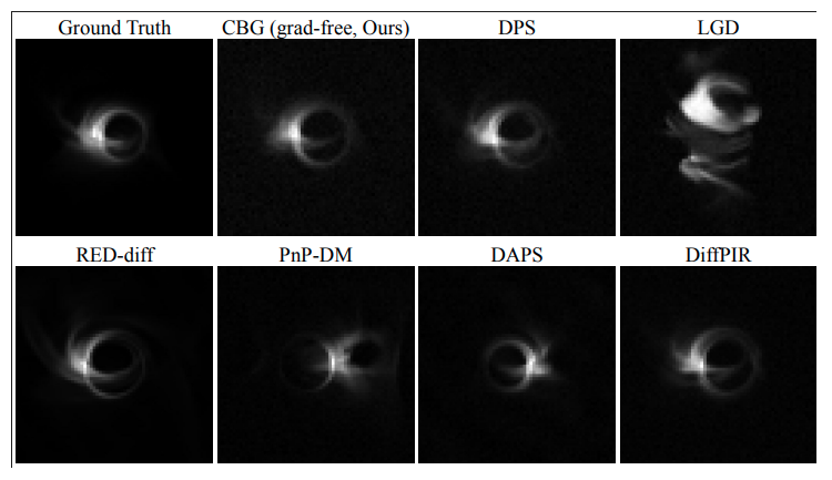
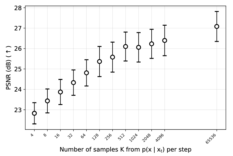
We apply CBG to a scientific inverse problem: reconstructing black-hole images from radio-telescope measurements. The pretrained diffusion model acts as an image prior, while the measurement model supplies the likelihood. Using the gradient-free estimator, CBG produces reconstructions that remain visually consistent with the ground truth and reaches stronger PSNR as the number of per-step denoising candidates increases.

Black-hole imaging reconstruction results
Uncurated comparison of CBG+DDPM with other test-time guidance methods for the black-hole imaging task. Despite computing no likelihood gradient, gradient-free CBG reconstructs the ground truth samples well.
Black-hole imaging increasing K
Increasing the number of samples \(K\) per denoising step consistently increases PSNR for the black-hole imaging task.

Image Inverse Problems

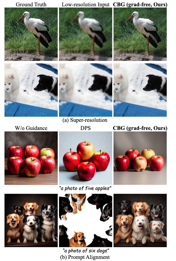
We also apply CBG to two image tasks: 4x super-resolution and prompt alignment. In super-resolution, CBG reconstructs 256 × 256 images from 64 × 64 inputs by treating the low-resolution observation as a likelihood. In prompt alignment, CBG uses a vision-language reward model as \(r(x; y)\) to guide text-to-image generation toward exact prompt constraints.

Image inverse problem results for super-resolution and prompt alignment
Image inverse problems: CBG applies to super-resolution and prompt alignment, reconstructing high-resolution images and satisfying exact object-count constraints.

Citation

BibTeX

@inproceedings{geyfman2026calibrated,
  title     = {Calibrated Test-Time Guidance for Bayesian Inference},
  author    = {Geyfman, Daniel and Draxler, Felix and Groeneveld, Jan and Lee, Hyunsoo and Karaletsos, Theofanis and Mandt, Stephan},
  booktitle = {International Conference on Machine Learning (ICML)},
  year      = {2026},
}